
Previously I showed how it was possible to obtain sunrise and sunset times for a whole year at any location on Earth, from a public source.
This time I am going to explain how to fetch that data, clean it up and create graphical visualizations like the one below, all using Python. A Jupyter Notebook is available on GitHub. Such data might even be useful in, for example, simulation of solar power generation.
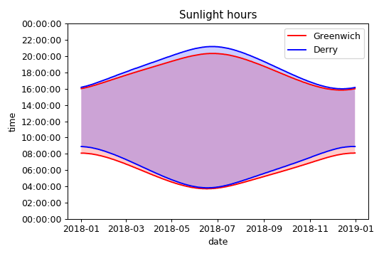 Sunlight hours for Derry vs Greenwich
Fetching the data
Looking at the URL string of the returned data query on the USNO website we can see that it contains all of the required values for longitude and latitude, as well as the place name label that we defined ourselves:
We can try replacing those values and expect to be able to retrieve any data set without going through the web interface. This makes it really easy to do what is known as web scraping, i.e. fetching the remote data table for any location automatically from our Python script. All we have to do is supply a label, and the coordinate values, and we can crudely modify the original URL to get the desired result.
url = "http://aa.usno.navy.mil/cgi-bin/aa_rstablew.pl?ID=AA&year=2018&task=0&place=%s&lon_sign=-1&lon_deg=%s&lon_min=%s&lat_sign=1&lat_deg=%s&lat_min=%s&tz=&tz_sign=-1" % (label, longitude[0], longitude[1], latitude[0], latitude[1])
urllib.urlretrieve (url, inFile)
When you fetch in this way a HTML file is returned, containing some html tags and some css code. But luckily the data we want is in plain text starting and ending at consistent line numbers each time, so we can read in the file, slice the lines that we want and then re-save the local file wth only the trimmed data.
# Dirty and dumb way to get rid of the html and css before the data table:
f = open(inFile, 'r')
# Gets a list of all the lines in the file, with each line as an un-split string:
# Crucially, the line endings remain intact so the local file will be identical to the original raw text!
html=f.readlines()
f.close()
raw = html[25:66] # Slice only the lines that we need. This is hardcoded but was the best method I found.

# Create/OverWrite the local file:
with open(inFile, "w") as text_file:
	for line in raw:
		text_file.write(line)</pre>
Every time you run this code it fetches from the USNO website. If you plan to run this code many times for the same geographic location it is worth saving to a local file to give their web server a break!
Data wrangling
Now that we have a local data file, let’s read it in to Python. Not so fast! It took me a while to find the best method here. Normally, as a scientist, I work with tabular data containing floats, not a mix of data types. So I often use numpy.loadtxt() as my go to method for reading data files. However, if we try this we get an error:
A = np.loadtxt(inFile, skiprows=9) # Gives "ValueError: Wrong number of columns at line 38"</pre>
Numpy’s loadtxt() function does not like it when a file contains columns of different lengths. Let’s try a different way.
Let’s try a pandas-based approach first.
df = pd.read_csv(inFile, skiprows=range(9), header=None, infer_datetime_format=True)
print df, df.shape</pre>
This almost works, but we get a collection of rows where each row is a long string. It has not split the row strings into columns yet!
0
0   01  0805 1602  0738 1649  0645 1740  0536 1833...
1   02  0805 1603  0737 1651  0643 1742  0533 1835...
2   03  0805 1604  0735 1653  0641 1744  0531 1836...
3   04  0805 1605  0734 1655  0639 1745  0529 1838...
4   05  0805 1606  0732 1657  0637 1747  0527 1840...
5   06  0804 1608  0730 1659  0635 1749  0524 1841...
6   07  0804 1609  0729 1700  0632 1751  0522 1843...
7   08  0803 1610  0727 1702  0630 1752  0520 1845...
8   09  0803 1612  0725 1704  0628 1754  0518 1846...
9   10  0802 1613  0723 1706  0626 1756  0516 1848...
10  11  0802 1614  0721 1708  0623 1758  0513 1850...
11  12  0801 1616  0720 1710  0621 1759  0511 1851...
12  13  0800 1617  0718 1711  0619 1801  0509 1853...
13  14  0800 1619  0716 1713  0617 1803  0507 1855...
14  15  0759 1620  0714 1715  0614 1804  0505 1856...
15  16  0758 1622  0712 1717  0612 1806  0503 1858...
16  17  0757 1624  0710 1719  0610 1808  0500 1900...
17  18  0756 1625  0708 1720  0608 1810  0458 1901...
18  19  0755 1627  0706 1722  0605 1811  0456 1903...
19  20  0754 1628  0704 1724  0603 1813  0454 1905...
20  21  0753 1630  0702 1726  0601 1815  0452 1906...
21  22  0752 1632  0700 1728  0559 1816  0450 1908...
22  23  0751 1634  0658 1729  0556 1818  0448 1910...
23  24  0749 1635  0656 1731  0554 1820  0446 1911...
24  25  0748 1637  0654 1733  0552 1821  0444 1913...
25  26  0747 1639  0652 1735  0549 1823  0442 1915...
26  27  0746 1641  0650 1737  0547 1825  0440 1916...
27  28  0744 1642  0648 1738  0545 1826  0438 1918...
28  29  0743 1644             0543 1828  0436 1920...
29  30  0741 1646             0540 1830  0434 1921...
30  31  0740 1648             0538 1831           ...
(31, 1)
In order to manipulate the data we would like Pandas to delimit the data correctly into rows and columns, and in this case we have whitespace between them.
df = pd.read_csv(inFile, skiprows=range(9), header=None, delim_whitespace=True, infer_datetime_format=True)</pre>
This does not produce the desired results, because the columns get shifted to the left to fill in the empty gaps of shorter months, e.g. now February has 31 days!
0    1     2    3     4    5     6    7     8    9    ...       15  \
0    1  805  1602  738  1649  645  1740  536  1833  432   ...    424.0
1    2  805  1603  737  1651  643  1742  533  1835  430   ...    425.0
2    3  805  1604  735  1653  641  1744  531  1836  429   ...    427.0
3    4  805  1605  734  1655  639  1745  529  1838  427   ...    428.0
4    5  805  1606  732  1657  637  1747  527  1840  425   ...    430.0
5    6  804  1608  730  1659  635  1749  524  1841  423   ...    431.0
6    7  804  1609  729  1700  632  1751  522  1843  421   ...    433.0
7    8  803  1610  727  1702  630  1752  520  1845  420   ...    434.0
8    9  803  1612  725  1704  628  1754  518  1846  418   ...    436.0
9   10  802  1613  723  1706  626  1756  516  1848  416   ...    438.0
10  11  802  1614  721  1708  623  1758  513  1850  415   ...    439.0
11  12  801  1616  720  1710  621  1759  511  1851  413   ...    441.0
12  13  800  1617  718  1711  619  1801  509  1853  412   ...    442.0
13  14  800  1619  716  1713  617  1803  507  1855  410   ...    444.0
14  15  759  1620  714  1715  614  1804  505  1856  409   ...    445.0
15  16  758  1622  712  1717  612  1806  503  1858  407   ...    447.0
16  17  757  1624  710  1719  610  1808  500  1900  406   ...    449.0
17  18  756  1625  708  1720  608  1810  458  1901  404   ...    450.0
18  19  755  1627  706  1722  605  1811  456  1903  403   ...    452.0
19  20  754  1628  704  1724  603  1813  454  1905  402   ...    453.0
20  21  753  1630  702  1726  601  1815  452  1906  400   ...    455.0
21  22  752  1632  700  1728  559  1816  450  1908  359   ...    457.0
22  23  751  1634  658  1729  556  1818  448  1910  358   ...    458.0
23  24  749  1635  656  1731  554  1820  446  1911  357   ...    500.0
24  25  748  1637  654  1733  552  1821  444  1913  356   ...    501.0
25  26  747  1639  652  1735  549  1823  442  1915  354   ...    503.0
26  27  746  1641  650  1737  547  1825  440  1916  353   ...    504.0
27  28  744  1642  648  1738  545  1826  438  1918  352   ...    506.0
28  29  743  1644  543  1828  436  1920  351  2004  346   ...    557.0
29  30  741  1646  540  1830  434  1921  351  2005  347   ...    559.0
30  31  740  1648  538  1831  350  2006  422  1950  511   ...      NaN

		16     17      18     19      20     21      22     23      24
0   1948.0  512.0  1847.0  600.0  1738.0  653.0  1633.0  743.0  1555.0
1   1946.0  514.0  1844.0  602.0  1736.0  655.0  1631.0  744.0  1554.0
2   1945.0  516.0  1842.0  604.0  1733.0  657.0  1630.0  746.0  1554.0
3   1943.0  517.0  1840.0  605.0  1731.0  658.0  1628.0  747.0  1553.0
4   1941.0  519.0  1838.0  607.0  1729.0  700.0  1626.0  748.0  1553.0
5   1939.0  520.0  1835.0  609.0  1727.0  702.0  1625.0  750.0  1552.0
6   1938.0  522.0  1833.0  610.0  1724.0  704.0  1623.0  751.0  1552.0
7   1936.0  524.0  1831.0  612.0  1722.0  706.0  1621.0  752.0  1552.0
8   1934.0  525.0  1828.0  614.0  1720.0  707.0  1620.0  753.0  1551.0
9   1932.0  527.0  1826.0  615.0  1718.0  709.0  1618.0  754.0  1551.0
10  1930.0  528.0  1824.0  617.0  1716.0  711.0  1617.0  755.0  1551.0
11  1928.0  530.0  1822.0  619.0  1713.0  712.0  1615.0  756.0  1551.0
12  1926.0  532.0  1819.0  620.0  1711.0  714.0  1614.0  757.0  1551.0
13  1924.0  533.0  1817.0  622.0  1709.0  716.0  1612.0  758.0  1551.0
14  1923.0  535.0  1815.0  624.0  1707.0  718.0  1611.0  759.0  1551.0
15  1921.0  536.0  1812.0  625.0  1705.0  719.0  1610.0  800.0  1551.0
16  1918.0  538.0  1810.0  627.0  1703.0  721.0  1608.0  800.0  1552.0
17  1916.0  539.0  1808.0  629.0  1701.0  723.0  1607.0  801.0  1552.0
18  1914.0  541.0  1806.0  631.0  1659.0  724.0  1606.0  802.0  1552.0
19  1912.0  543.0  1803.0  632.0  1657.0  726.0  1605.0  802.0  1553.0
20  1910.0  544.0  1801.0  634.0  1655.0  728.0  1603.0  803.0  1553.0
21  1908.0  546.0  1759.0  636.0  1652.0  729.0  1602.0  803.0  1554.0
22  1906.0  547.0  1756.0  637.0  1650.0  731.0  1601.0  804.0  1554.0
23  1904.0  549.0  1754.0  639.0  1648.0  733.0  1600.0  804.0  1555.0
24  1902.0  551.0  1752.0  641.0  1647.0  734.0  1559.0  805.0  1555.0
25  1900.0  552.0  1749.0  643.0  1645.0  736.0  1559.0  805.0  1556.0
26  1858.0  554.0  1747.0  644.0  1643.0  737.0  1558.0  805.0  1557.0
27  1855.0  556.0  1745.0  646.0  1641.0  739.0  1557.0  805.0  1558.0
28  1743.0  648.0  1639.0  740.0  1556.0  805.0  1559.0    NaN     NaN
29  1740.0  650.0  1637.0  742.0  1555.0  806.0  1600.0    NaN     NaN
30     NaN    NaN     NaN    NaN     NaN    NaN     NaN    NaN     NaN

[31 rows x 25 columns]
Since we notice that the tabular data has regular, repeating columnar widths, we can use the Pandas fixed width file function read_fwf(). Here is an example for two columns.
eg = pd.read_fwf(inFile, colspecs=[(4,8), (9,13)], skiprows=9, header=None)
We can adapt this approach to get all columns. Notice that not each column width is identical but they are bunched in a way that we can use. We can straight away loop through the relevant columns for sunrise and sunset and store them in separate Pandas dataframes.
sunrise = pd.read_fwf(inFile, colspecs=[(i, i+4) for i in range(4,132,11)], skiprows=9, header=None).values.T.flatten()
sunset  = pd.read_fwf(inFile, colspecs=[(i, i+4) for i in range(9,137,11)], skiprows=9, header=None).values.T.flatten()
# Remove all NaNs from the flattened lists to leave just the days that exist: https://stackoverflow.com/questions/11620914/removing-nan-values-from-an-array
sunrise = sunrise[~np.isnan(sunrise)].astype('int').tolist()
sunset = sunset[~np.isnan(sunset)].astype('int').tolist()
I have also transposed and flattened the data, then removed any NaN values and converted to lists, so that we have a list of 365 sunrise times and a list of 365 sunset times. Notice that all of the methods presented here should account for leap years, which contain 366 days, automatically!
Now we want to convert our float values to datetimes. We can do this using Python’s datetime module but we will need to give it integer values for hours, minutes and seconds.
srise = [datetime.time(int(str(a)[:-2]), int(str(a)[-2:]), 0) for a in sunrise]
sset = [datetime.time(int(str(a)[:-2]), int(str(a)[-2:]), 0) for a in sunset]
Creating a date list
Our method for extracting the sunrise and sunset times didn’t preserve the dates on which those values occurred, but we can easily create one. Pandas can create a period list using the date_range function, and this can be converted to datetimes.
periodlist = pd.date_range(start='%s-01-01' % year, end='%s-12-31' % year, freq='D')
print periodlist

datelist = [pd.to_datetime(date, format='%m-%d').date() for date in periodlist]
print "Datelist:\n", datelist[:10]
This datelist will allow us to plot our sunrise and sunset times against the day of the year easily.
Visualization
Now we can simply invoke matplotlib, creating line plots for the sunrise and sunset data series’ and filling in between using the fill_between() method.
# Create a nice plot:
plt.close()
plt.figure()

# Plot the sunrise and sunset series as lineplots:
plt.plot(datelist, srise, label='sunrise')
plt.plot(datelist, sset, label='sunset')

# Let's put a fill between the two line plots:
plt.fill_between(datelist, srise, sset, facecolor='yellow', alpha=0.2, interpolate=True)

plt.title('Sunlight hours')
plt.xlabel('date')

# Make sure the y axis covers the (almost) full range of 24 hours:
plt.ylim([datetime.time.min, datetime.time.max])
# The above y limits do not force the y axis to run a full 24 hours, so force manual axes tick values.
# Give a range of values in seconds and matplotlib is clever enough to work it out:
plt.yticks(range(0, 60*60*25, 2*60*60))

plt.legend()
plt.savefig('working.png', dpi=90)
plt.show()
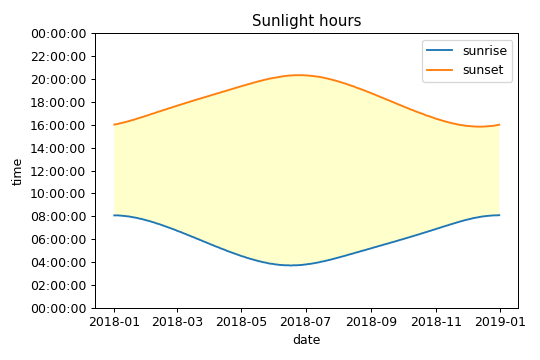 Figure: Data for Greenwich, UK, visualized from USNO data.
Final code
In my final code I added some additional features such as a location dictionary, that allows me to compare a daylight times for different locations on a single plot. My final code can be found in a Jupyter Notebook, which is available on GitHub. Here is a comparison between Greenwich, UK and Derry, UK.
Figure: Sunlight hours for Derry vs Greenwich
As we can see, in winter the two locations have identical sunset times but the sunrise in Derry is significantly later. In summer The sunrise times are similar, but Derry has a much later sunset. The days in Derry are really short in winter and really long in summer, as the locals will tell you! As one of the farthest North-Westerly cities in the UK, Derry is considerably further north and further west than Greenwich (London), but it is still in the same time zone. Note that I have not included Daylight saving times in my code. Times are all in GMT.
 Figure: Map showing Derry and Greenwich (London), UK.