Deriving Snell’s Law
One of the most elegant results in optics is Snell’s Law, which relates the angles of incidence and refraction at the boundary between two media:
$$ n_1 \sin\theta_1 = n_2 \sin\theta_2. $$
Many textbooks derive this result using constrained optimization and Lagrange multipliers. However, there is a simpler and more intuitive approach: eliminate the constraint through substitution and reduce the problem to an ordinary single-variable minimization.
This derivation follows directly from Fermat’s Principle, which states that light follows a path for which the optical path length is stationary (typically a minimum).
The Geometry
Consider two points, $A$ and $C$, separated by an interface between media with refractive indices $n_1$ and $n_2$.
Light travels:
- From $A$ to the interface at $B$
- From $B$ to $C$
The distances perpendicular to the interface are $d_1$ and $d_2$, respectively.
The ray makes angles $\theta_1$ and $\theta_2$ with the normal in the two media.
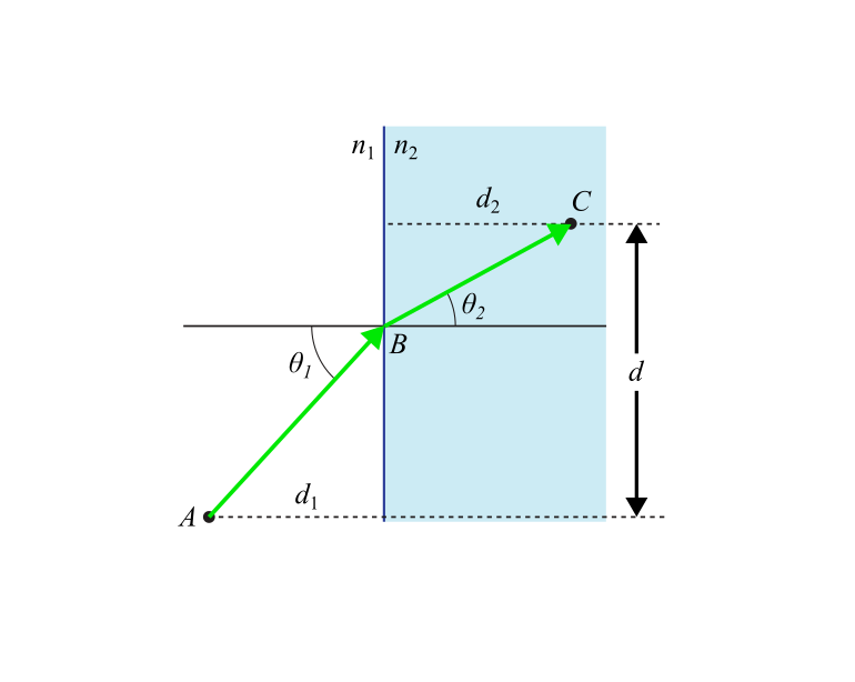 (Image adapted from Saleh & Teich “Fundamentals of Optics”, 3rd edition (Wiley), where the derivation of Snell’s Law is left as an exercise for the reader.)
Step 1: Write the Optical Path Length
The optical path length is
$$ L = n_1 AB + n_2 BC. $$
From the geometry,
$$ AB = d_1 \sec\theta_1, $$
and
$$ BC = d_2 \sec\theta_2. $$
Therefore
$$ L = n_1 d_1 \sec\theta_1 + n_2 d_2 \sec\theta_2. $$
The geometry also imposes the constraint
$$ d_1\tan\theta_1 + d_2\tan\theta_2 = d, $$
where $d$ is the total horizontal displacement between $A$ and $C$.
Step 2: Eliminate the Constraint
Introduce a new variable
$$ x = d_1\tan\theta_1. $$
Geometrically, $x$ is simply the horizontal position of the refraction point $B$.
The constraint becomes
$$ d_2\tan\theta_2 = d - x, $$
so that
$$ \tan\theta_1 = \frac{x}{d_1}, \qquad \tan\theta_2 = \frac{d-x}{d_2}. $$
Using
$$ \sec\theta = \sqrt{1+\tan^2\theta}, $$
we obtain
$$ AB = d_1\sqrt{1+\frac{x^2}{d_1^2}} = \sqrt{d_1^2+x^2} $$
and
$$ BC = d_2\sqrt{1+\frac{(d-x)^2}{d_2^2}} = \sqrt{d_2^2+(d-x)^2}. $$
Substituting into the optical path length gives
$$ L(x) = n_1\sqrt{d_1^2+x^2} + n_2\sqrt{d_2^2+(d-x)^2}. $$
The constrained optimization problem has now become an ordinary one-dimensional minimization.
Step 3: Differentiate
Differentiate with respect to $x$:
$$ \frac{dL}{dx} = n_1\frac{x}{\sqrt{d_1^2+x^2}} - n_2\frac{d-x}{\sqrt{d_2^2+(d-x)^2}}. $$
At the optimum path,
$$ \frac{dL}{dx}=0, $$
which gives
$$ n_1\frac{x}{\sqrt{d_1^2+x^2}} = n_2\frac{d-x}{\sqrt{d_2^2+(d-x)^2}}. $$
Step 4: Recognize the Sines
Looking back at the geometry,
$$ \sin\theta_1 = \frac{x}{\sqrt{d_1^2+x^2}}, $$
and
$$ \sin\theta_2 = \frac{d-x} {\sqrt{d_2^2+(d-x)^2}}. $$
Substituting these expressions into the stationarity condition yields
$$ n_1\sin\theta_1 = n_2\sin\theta_2. $$
This is exactly Snell’s Law.
Why This Approach Is Nice
Many presentations formulate the problem as
$$ \text{minimize }n_1 d_1 \sec\theta_1 + n_2 d_2 \sec\theta_2 $$
subject to the constraint
$$ d_1\tan\theta_1+d_2\tan\theta_2=d. $$
and then solve it using a Lagrange multiplier.
While perfectly valid, the constraint has a clear geometric meaning: it merely specifies where the ray crosses the interface. By introducing the crossing position $x$ directly, the constraint disappears entirely.
The derivation then becomes:
- Express the optical path length as a function of $x$.
- Differentiate.
- Set the derivative equal to zero.
- Recognize the resulting terms as $\sin\theta_1$ and $\sin\theta_2$.
The result follows in just a few lines of algebra.
But Aren’t We Ignoring a Variable?
When first encountering substitution, many students have an understandable concern:
We started with two variables, $\theta_1$ and $\theta_2$. After substitution, one of them seems to disappear. Aren’t we ignoring its effect?
The answer is no.
The crucial insight is that once the constraint
$$ d_1\tan\theta_1 + d_2\tan\theta_2 = d $$
is imposed, the two angles are no longer free to vary independently.
If $\theta_1$ changes, then $\theta_2$ must change as well.
The constraint couples them together.
As a consequence, although we have written down two variables, the system has only one independent degree of freedom.
Substitution does not throw away a variable.
It simply replaces several dependent variables with a smaller set of independent variables.
Variables Versus Degrees of Freedom
This is one of the most important conceptual ideas in mathematics and physics:
Variables are not the same thing as degrees of freedom.
At first sight, the problem appears to contain two variables:
$$ (\theta_1,\theta_2). $$
However, the constraint restricts the allowed values to a one-dimensional curve:
$$ d_1\tan\theta_1+d_2\tan\theta_2=d. $$
Geometrically, the pair $(\theta_1,\theta_2)$ cannot explore the entire plane.
Instead, all physically allowed solutions must lie somewhere along a single curve.
All possible (θ₁, θ₂)
          ↓
   Apply constraint
          ↓
     Allowed curve
          ↓
 One degree of freedom
The substitution
$$ x=d_1\tan\theta_1 $$
simply provides a convenient coordinate along that curve.
A Train-on-a-Track Analogy
A useful analogy from classical mechanics is a train constrained to move along a railway track.
In open space, a vehicle might be described by two coordinates:
$$ (x,y). $$
Both are needed because the vehicle is free to move in two directions.
Now place the vehicle on a railway track.
The train can move only forward or backward along the track.
Although the coordinates $(x,y)$ still exist, they are no longer independent.
Once we know the distance $s$ traveled along the track, both coordinates are fixed:
$$ x=x(s), \qquad y=y(s). $$
Moving the train changes both $x$ and $y$, but neither changes independently.
The single parameter $s$ captures all possible motion.
Substitution works in exactly the same way. We describe the system using the true degree of freedom rather than an oversized set of constrained coordinates.
Where Did the Missing Variable Go?
The “missing” variable has not actually disappeared.
Its influence has been absorbed into the remaining variable.
A simple example makes this clear.
Consider
$$ f(x,y)=x^2+y^2 $$
with the constraint
$$ y=2x. $$
Substituting gives
$$ F(x) = x^2+(2x)^2 = 5x^2. $$
Differentiating,
$$ \frac{dF}{dx}=10x. $$
At first glance, the contribution from $y$ appears to have vanished.
But the chain rule tells the full story:
$$ \frac{dF}{dx} = \frac{\partial f}{\partial x} + \frac{\partial f}{\partial y} \frac{dy}{dx}. $$
The dependence on $y$ is still there.
It enters through
$$ \frac{dy}{dx}. $$
Substitution doesn’t ignore the second variable, it automatically includes its response through the constraint.
Returning to Snell’s Law
In the refraction problem, the position of the crossing point $B$ uniquely determines the ray.
Once $B$ is fixed:
- $\theta_1$ is fixed.
- $\theta_2$ is fixed.
- The optical path length is fixed.
The problem therefore has only one true degree of freedom.
Instead of describing the ray with two coupled angles, we describe it using the position of the interface crossing point:
$$ x=d_1\tan\theta_1. $$
This is not merely an algebraic trick. It is a better coordinate system for the underlying geometry.
A Broader Lesson
One of the deepest ideas in mathematics and theoretical physics is that:
Good substitutions reveal the true degrees of freedom.
This idea appears everywhere:
- A bead constrained to move on a wire is best described by distance along the wire.
- Circular motion is often simpler in polar coordinates than Cartesian coordinates.
- Mechanical systems are frequently described using generalized coordinates chosen to automatically satisfy constraints.
- Electromagnetic waveguides are often described using modal amplitudes rather than field values at every point.
- In optics, the refraction problem becomes simpler when we describe the ray by the position where it crosses the interface.
Viewed this way, substitution is far more than a computational shortcut.
It is the art of finding a coordinate system that matches the geometry and physics of the problem.
Final Result
Starting from Fermat’s Principle and minimizing the optical path length,
$$ L(x) = n_1\sqrt{d_1^2+x^2} + n_2\sqrt{d_2^2+(d-x)^2}, $$
we obtain
$$ \boxed{ n_1\sin\theta_1 =n_2\sin\theta_2 } $$
which is precisely Snell’s Law.
More importantly, the derivation illustrates a broader lesson: when constraints are present, the most natural way to solve a problem is often to replace dependent variables with the true degrees of freedom. The resulting mathematics is usually simpler, and the underlying physics becomes easier to see.
[ Disclaimer - I used an LLM to help me write some parts of this blog post]